10 Data Sets

Note

Chapter 10 demonstrates several, though not all, data objects from package datasets (R version 4.5.3 (2026-03-11)) and package spatstat.data (v3.1.9, GPL (>= 2)).

The function calls in Chapter 10 are exclusively those provided in package base and stats (R version 4.5.3 (2026-03-11)), and in the spatstat.* family of packages.

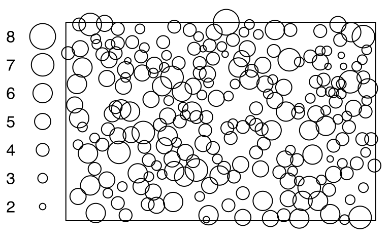
10.1 `anemones`

The point-pattern (ppp.object, Chapter 36) anemones from package spatstat.data (v3.1.9, GPL (>= 2)) has (Listing 10.2, Figure 10.1)

231 points (Listing 10.3);
rectangle observation window (Chapter 34, Listing 10.4);
one integer-mark (Listing 10.5);
'vector' mark-format (Listing 10.6).

Listing 10.1: Figure: anemones

Code

par(mar = c(0,0,0,0))
spatstat.data::anemones |>
  spatstat.geom::plot.ppp(main = NULL)

Listing 10.2: Data: anemones

spatstat.data::anemones |>
  spatstat.geom::print.ppp()
# Marked planar point pattern: 231 points
# marks are numeric, of storage type  'integer'
# window: rectangle = [0, 280] x [0, 180] units

Listing 10.3: Review: number of points in anemones

spatstat.data::anemones |>
  spatstat.geom::npoints.ppp()
# [1] 231

Listing 10.4: Review: window of anemones

spatstat.data::anemones |>
  spatstat.geom::Window.ppp()
# window: rectangle = [0, 280] x [0, 180] units

Listing 10.5: Review: storage mode of the marks of anemones

spatstat.data::anemones |>
  spatstat.geom::marks.ppp() |>
  typeof()
# [1] "integer"

Listing 10.6: Review: mark-format of anemones

spatstat.data::anemones |>
  spatstat.geom::markformat.ppp()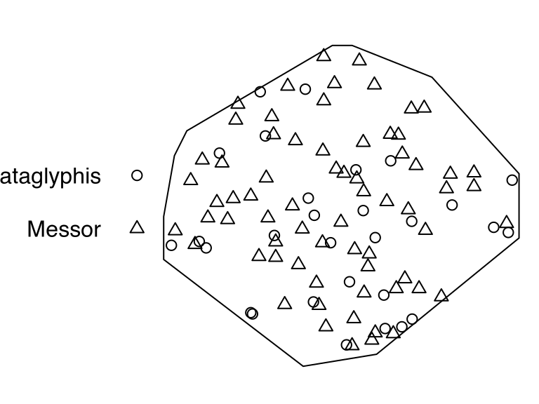
# [1] "vector"

10.2 `ants`

The point-pattern (ppp.object, Chapter 36) ants from package spatstat.data (v3.1.9, GPL (>= 2)) has (Listing 10.8, Figure 10.2)

97 points;
polygonal window;
one multi-type mark with two levels, 'Cataglyphis' and 'Messor' (Listing 10.9);
'vector' mark-format.

Listing 10.7: Figure: ants

Code

par(mar = c(0,0,0,0))
spatstat.data::ants |>
  spatstat.geom::plot.ppp(main = NULL)

Listing 10.8: Data: ants

spatstat.data::ants |>
  spatstat.geom::print.ppp()
# Marked planar point pattern: 97 points
# Multitype, with levels = Cataglyphis, Messor 
# window: polygonal boundary
# enclosing rectangle: [-25, 803] x [-49, 717] units (one unit = 0.5 feet)

Listing 10.9: Review: marks of ants

spatstat.data::ants |>
  spatstat.geom::marks.ppp() |>
  table()
# 
# Cataglyphis      Messor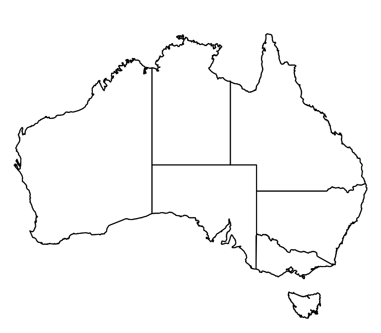 
#          29          68

10.3 `austates`

The tessellation (Chapter 42) austates from package spatstat.data (v3.1.9, GPL (>= 2)) has (Listing 10.11, Figure 10.3)

7 tiles (Listing 10.12);
polygonal window;
no marks.

Listing 10.10: Figure: austates

Code

par(mar = c(0,0,1,0))
spatstat.data::austates |>
  spatstat.geom::plot.tess(main = '')

Listing 10.11: Data: austates

spatstat.data::austates |>
  spatstat.geom::print.tess()
# Tessellation
# Tiles are irregular polygons
# 7 tiles (irregular windows)
# window: polygonal boundary
# enclosing rectangle: [113.19392, 153.6692] x [-43.59316, -10.93156] degrees

Listing 10.12: Review: tiles in austates

spatstat.data::austates |>
  spatstat.geom::tiles()
# List of spatial objects
# 
# WA:
# window: polygonal boundary
# enclosing rectangle: [113.19392, 129.01141] x [-35.11407, -13.76426] degrees
# 
# NT:
# window: polygonal boundary
# enclosing rectangle: [129.01141, 138.0038] x [-25.988593, -11.045627] degrees
# 
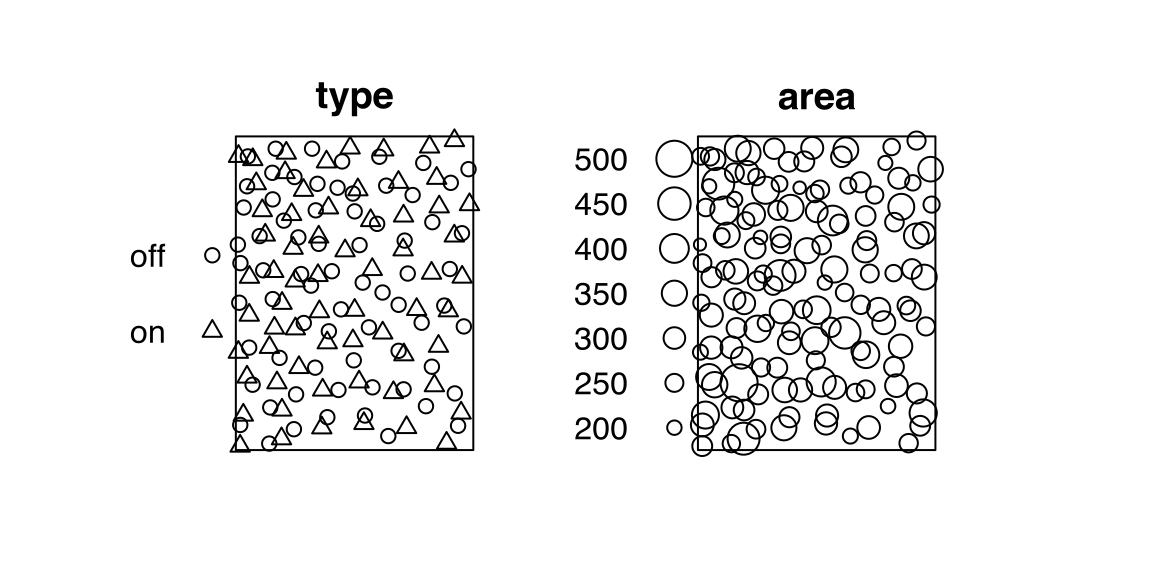
# ✂️ --- output truncated --- ✂️

10.4 `betacells`

The point-pattern (ppp.object, Chapter 36) betacells from package spatstat.data (v3.1.9, GPL (>= 2)) has (Listing 10.14, Figure 10.4)

135 points;
rectangle window;
'dataframe' mark-format (Listing 10.15);
one numeric mark area (Listing 10.16);
one multi-type mark type with two levels, 'off' and 'on' (Listing 10.16).

Listing 10.13: Figure: betacells

Code

par(mar = c(0,0,0,0))
spatstat.data::betacells |>
  spatstat.geom::plot.ppp(main = '')

Listing 10.14: Data: betacells

spatstat.data::betacells |>
  spatstat.geom::print.ppp()
# Marked planar point pattern: 135 points
# Mark variables: type, area 
# window: rectangle = [28.08, 778.08] x [16.2, 1007.02] microns

Listing 10.15: Review: mark-format of betacells

spatstat.data::betacells |>
  spatstat.geom::markformat.ppp()
# [1] "dataframe"

Listing 10.16: Review: marks of betacells

spatstat.data::betacells |>
  spatstat.geom::marks.ppp()
#     type  area
# 1     on 275.9
# 2    off 241.2
# 3     on 256.0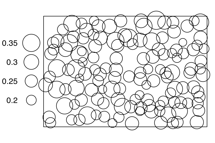
# ✂️ --- output truncated --- ✂️

10.5 `bronzefilter`

The point-pattern (ppp.object, Chapter 36) bronzefilter from package spatstat.data (v3.1.9, GPL (>= 2)) has (Listing 10.18, Figure 10.5)

678 points;
rectangle window;
one numeric mark.

Listing 10.17: Figure: bronzefilter

Code

par(mar = c(0,1,0,0))
spatstat.data::bronzefilter |>
  spatstat.geom::plot.ppp(main = NULL)

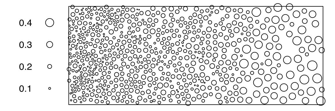
Listing 10.18: Data: bronzefilter

spatstat.data::bronzefilter |>
  spatstat.geom::print.ppp()
# Marked planar point pattern: 678 points
# marks are numeric, of storage type  'double'
# window: rectangle = [0, 18] x [0, 7] mm

10.6 `btb.extra`

The point-pattern-list (ppplist, Chapter 37) btb.extra from package spatstat.data (v3.1.9, GPL (>= 2)) (Listing 10.20, Figure 10.6)

inherits from the S3 class 'solist' (Chapter 39, Listing 10.21);
contains 2 point-pattern (ppp.object, Chapter 36) members (Listing 10.22).

Listing 10.19: Figure: btb.extra

Code

par(mar = c(0,1,1,1))
spatstat.data::btb.extra |> 
  spatstat.geom::plot.solist()

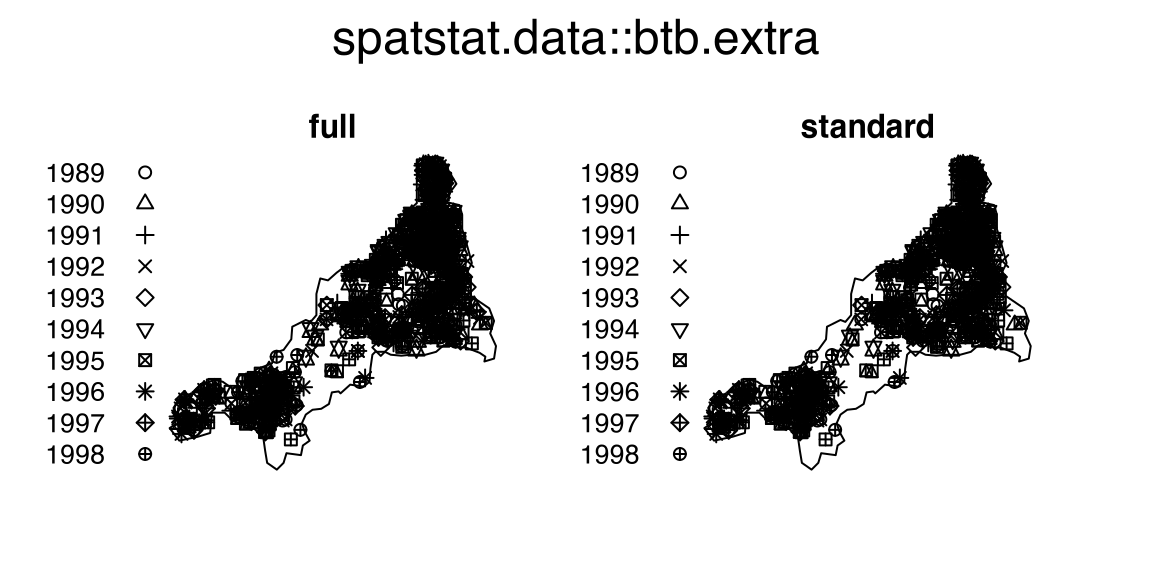
Listing 10.20: Data: btb.extra

spatstat.data::btb.extra
# List of point patterns
# 
# full:
# Marked planar point pattern: 919 points
# Mark variables: year, spoligotype 
# window: polygonal boundary
# enclosing rectangle: [133.5147, 246.0193] x [10.88514, 118.7298] km
# 
# standard:
# Marked planar point pattern: 873 points
# Mark variables: year, spoligotype 
# window: polygonal boundary
# enclosing rectangle: [133.5147, 246.0193] x [10.88514, 118.7298] km

Listing 10.21: Review: inheritance of btb.extra

spatstat.data::btb.extra |> 
  class()
# [1] "ppplist" "solist"  "anylist" "listof"  "list"

Listing 10.22: Review: class of members of btb.extra

spatstat.data::btb.extra |> 
  sapply(FUN = class)
#     full standard 
#    "ppp"    "ppp"

10.7 `cars`

The data frame (data.frame, Chapter 18) cars from package datasets (R version 4.5.3 (2026-03-11)) has (Listing 10.23)

50 rows and 2 columns (Listing 10.24)
two numeric columns: $speed and $dist.

Listing 10.23: Data: cars

datasets::cars |>
  print.data.frame()
#    speed dist
# 1      4    2
# 2      4   10
# 3      7    4
# 4      7   22
# ✂️ --- output truncated --- ✂️

Listing 10.24: Review: dimensions of cars

datasets::cars |>
  dim.data.frame()
# [1] 50  2

10.8 `cetaceans`

The hyper data frame (hyperframe, Chapter 26) cetaceans from package spatstat.data (v3.1.9, GPL (>= 2)) has (Listing 10.25)

9 rows and 4 (hyper)columns (Listing 10.26)
four point-pattern (ppp, Chapter 36) hypercolumns: $whales, $dolphins, $fish and $plankton.

Listing 10.25: Data: cetaceans

spatstat.data::cetaceans |>
  spatstat.geom::print.hyperframe()
# Hyperframe:
#   whales dolphins  fish plankton
# 1  (ppp)    (ppp) (ppp)    (ppp)
# 2  (ppp)    (ppp) (ppp)    (ppp)
# 3  (ppp)    (ppp) (ppp)    (ppp)
# ✂️ --- output truncated --- ✂️

Listing 10.26: Review: dimensions of cetaceans

spatstat.data::cetaceans |>
  spatstat.geom::dim.hyperframe()
# [1] 9 4

10.9 `demohyper`

The hyper data frame (hyperframe, Chapter 26) demohyper from package spatstat.data (v3.1.9, GPL (>= 2)) has (Listing 10.27)

3 rows and 3 (hyper)columns (Listing 10.28)
a point-pattern (ppp, Chapter 36) hypercolumn $Points
a pixel-image (im, Chapter 28) hypercolumn $Image
a regular column $Group.

Listing 10.27: Data: demohyper

spatstat.data::demohyper |>
  spatstat.geom::print.hyperframe()
# Hyperframe:
#   Points Image Group
# 1  (ppp)  (im)     a
# 2  (ppp)  (im)     b
# 3  (ppp)  (im)     a

Listing 10.28: Review: dimensions of demohyper

spatstat.data::demohyper |>
  spatstat.geom::dim.hyperframe()
# [1] 3 3

To view the hyper data frame demohyper in a desired format, readers may call the S3 method spatstat.geom::print.hyperframe() explicitly (Listing 10.27). Alternatively, readers may call the S3 generic function print() by simply typing demohyper at the R console prompt and pressing Enter, after putting the package spatstat.geom (v3.7.3, GPL (>= 2))

either, in the search() path, by either one of the following approaches,
- using the function library(), e.g., library(spatstat.geom), which is called internally by the function require();
- using the function attachNamespace(), e.g., attachNamespace('spatstat.geom');
or, in the loadedNamespaces(), by either one of the following approaches,
- using the function loadNamespace(), e.g., loadNamespace('spatstat.geom'), which is called internally by the function requireNamespace();
- calling or evaluating any function in the package spatstat.geom (v3.7.3, GPL (>= 2)) explicitly with its namespace, e.g., spatstat.geom::dim.hyperframe to print the function itself, or Listing 10.28, Listing 10.29, etc.

The rest of Section 10.9 showcases the *.hyperframe() methods of the .Primitive S3 generic functions names() (Listing 10.29) and `$` (Listing 10.30, Listing 10.31).

Listing 10.29 finds the (hyper)column names of the hyper data frame demohyper,

Listing 10.29: Review: (hyper)column names of demohyper

spatstat.data::demohyper |>
  spatstat.geom::names.hyperframe()
# [1] "Points" "Image"  "Group"

Listing 10.30 and Listing 10.31 observe the ppp-hypercolumn $Points,

Listing 10.30: Review: ppp-hypercolumn $Points

spatstat.data::demohyper$Points |>
  class()
# [1] "ppplist" "solist"  "anylist" "listof"  "list"

Listing 10.31: Advanced: ppp-hypercolumn $Points, nerdy!

spatstat.data::demohyper |>
  spatstat.geom::`$.hyperframe`(name = 'Points') |> # nerdy!!
  identical(y = spatstat.data::demohyper$Points) |>
  stopifnot()

Listing 10.32 and Listing 10.33 find the first point-pattern element of the ppp-hypercolumn $Points,

Listing 10.32: Review: 1st point-pattern in ppp-hypercolumn $Points

demohyper_p1 = spatstat.data::demohyper$Points[[1L]] 
demohyper_p1 |>
  spatstat.geom::print.ppp()
# Planar point pattern: 104 points
# window: binary image mask
# 128 x 128 pixel array (ny, nx)
# enclosing rectangle: [2.017, 3.93] x [0.645, 3.278] units

Listing 10.33: Advanced: 1st point-pattern in ppp-hypercolumn $Points, nerdy!

spatstat.data::demohyper$Points |>
  base::`[[`(i = 1L) |> # nerdy!!
  identical(y = demohyper_p1) |>
  stopifnot()

Listing 10.34 finds the first pixel-image element of the im-hypercolumn $Image,

Listing 10.34: Review: 1st pixel-image in im-hypercolumn $Image

spatstat.data::demohyper$Image[[1L]] |>
  spatstat.geom::print.im()
# real-valued pixel image
# 53 x 39 pixel array (ny, nx)
# enclosing rectangle: [2.017, 3.93] x [0.645, 3.278] units

10.10 `faithful`

The data frame (data.frame, Chapter 18) faithful from package datasets (R version 4.5.3 (2026-03-11)) has (Listing 10.35)

272 rows and 2 columns (Listing 10.36)
two numeric columns: $eruptions and $waiting.

Listing 10.35: Data: faithful

datasets::faithful |>
  print.data.frame()
#     eruptions waiting
# 1       3.600      79
# 2       1.800      54
# 3       3.333      74
# 4       2.283      62
# ✂️ --- output truncated --- ✂️

Listing 10.36: Review: dimensions of faithful

datasets::faithful |>
  dim.data.frame()
# [1] 272   2

10.11 `finpines`

The point-pattern (ppp.object, Chapter 36) finpines from package spatstat.data (v3.1.9, GPL (>= 2)) has (Listing 10.38, Figure 10.7)

126 points;
rectangle window;
two numeric marks, diameter and height.

Listing 10.37: Figure: finpines

Code

par(mar = c(0,0,0,0))
spatstat.data::finpines |>
  spatstat.geom::plot.ppp(main = '')

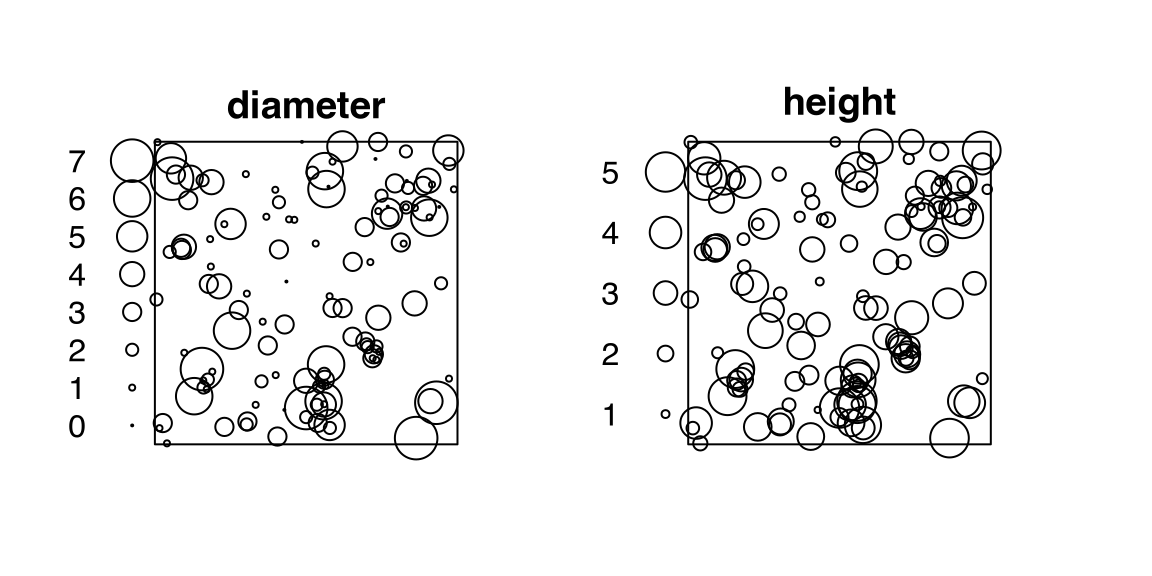
Listing 10.38: Data: finpines

spatstat.data::finpines |>
  spatstat.geom::print.ppp()
# Marked planar point pattern: 126 points
# Mark variables: diameter, height 
# window: rectangle = [-5, 5] x [-8, 2] metres

10.12 `flu`

The hyper data frame (hyperframe, Chapter 26) flu from package spatstat.data (v3.1.9, GPL (>= 2)) has (Listing 10.39)

41 rows and 4 (hyper)columns (Listing 10.40)
a point-pattern (ppp, Chapter 36) hypercolumn $pattern
regular columns $virustype, $stain, $frameid

Listing 10.39: Data: flu

spatstat.data::flu |>
  spatstat.geom::print.hyperframe()
# Hyperframe:
#                pattern virustype stain frameid
# wt M2-M1 13      (ppp)        wt M2-M1      13
# wt M2-M1 22      (ppp)        wt M2-M1      22
# wt M2-M1 27      (ppp)        wt M2-M1      27
# ✂️ --- output truncated --- ✂️

Listing 10.40: Review: dimensions of flu

spatstat.data::flu |>
  spatstat.geom::dim.hyperframe()
# [1] 41  4

10.13 `gorillas`

The point-pattern (ppp.object, Chapter 36) gorillas from package spatstat.data (v3.1.9, GPL (>= 2)) has (Listing 10.42, Figure 10.8)

647 points;
polygonal window;
two multi-type marks, group (with two levels 'major' and 'minor') and season (with two levels 'dry' and 'rainy').

Listing 10.41: Figure: gorillas

Code

par(mar = c(0,0,1,0))
spatstat.data::gorillas |>
  spatstat.geom::plot.ppp(which.marks = c('group', 'season'))

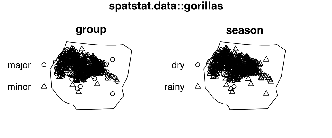
Listing 10.42: Data: gorillas

spatstat.data::gorillas |>
  spatstat.geom::print.ppp()
# Marked planar point pattern: 647 points
# Mark variables: group, season, date 
# window: polygonal boundary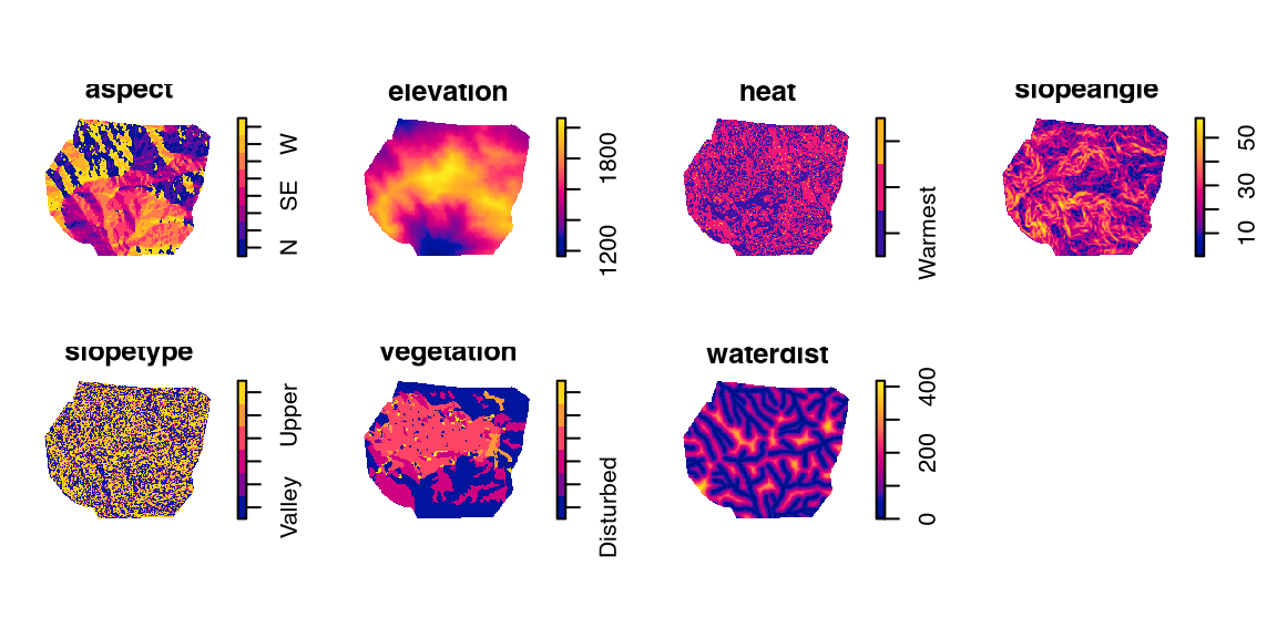
# enclosing rectangle: [580457.9, 585934] x [674172.8, 678739.2] metres

10.14 `gorillas.extra`

The pixel-image list (imlist, Chapter 29) gorillas.extra from package spatstat.data (v3.1.9, GPL (>= 2)) (Listing 10.44, Figure 10.9)

inherits from the S3 class 'solist' (Chapter 39, Listing 10.45);
contains 7 pixel-image (im, Chapter 28) members (Listing 10.46).

Listing 10.43: Figure: gorillas.extra

Code

par(mar = c(0,0,0,0))
spatstat.data::gorillas.extra |> 
  plot(main = '')

Listing 10.44: Data: gorillas.extra

spatstat.data::gorillas.extra
# List of pixel images
# 
# aspect:
# factor-valued pixel image
# factor levels:
# [1] "N"  "NE" "E"  "SE" "S"  "SW" "W"  "NW"
# 149 x 181 pixel array (ny, nx)
# enclosing rectangle: [580440, 586000] x [674160, 678730] metres
# 
# elevation:
# integer-valued pixel image
# 149 x 181 pixel array (ny, nx)
# enclosing rectangle: [580440, 586000] x [674160, 678730] metres
# 
# ✂️ --- output truncated --- ✂️

Listing 10.45: Review: inheritance of gorillas.extra

spatstat.data::gorillas.extra |> 
  class()
# [1] "imlist"  "solist"  "anylist" "listof"  "list"

Listing 10.46: Review: class of members of gorillas.extra

spatstat.data::gorillas.extra |> 
  sapply(FUN = class)
#     aspect  elevation       heat slopeangle  slopetype vegetation  waterdist 
#       "im"       "im"       "im"       "im"       "im"       "im"       "im"

10.15 `hyytiala`

The point-pattern (ppp.object, Chapter 36) hyytiala from package spatstat.data (v3.1.9, GPL (>= 2)) has (Listing 10.48, Figure 10.10)

168 points;
rectangle window;
one multi-type mark with four levels, 'aspen', 'birch', 'pine' and 'rowan' (Listing 10.49);
'vector' mark-format.

Listing 10.47: Figure: hyytiala

Code

par(mar = c(0,0,0,0))
spatstat.data::hyytiala |>
  spatstat.geom::plot.ppp(main = NULL)

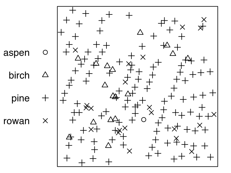
Listing 10.48: Data: hyytiala

spatstat.data::hyytiala |>
  spatstat.geom::print.ppp()
# Marked planar point pattern: 168 points
# Multitype, with levels = aspen, birch, pine, rowan 
# window: rectangle = [0, 20] x [0, 20] metres

Listing 10.49: Review: marks of hyytiala

spatstat.data::hyytiala |>
  spatstat.geom::marks.ppp() |>
  table()
# 
# aspen birch  pine rowan 
#     1    17   128    22

10.16 `Kovesi`

The hyper data frame (hyperframe, Chapter 26) Kovesi from package spatstat.data (v3.1.9, GPL (>= 2)) has (Listing 10.50)

41 rows and 13 (hyper)columns (Listing 10.51)
regular columns $linear, $diverging, etc.
a character hypercolumn $values. This is a length-41 (Listing 10.53) anylist (Chapter 15, Listing 10.52) of character vectors, each of them has a length of 256 (Listing 10.54).

Listing 10.50: Data: Kovesi

spatstat.data::Kovesi |>
  spatstat.geom::print.hyperframe()
# Hyperframe:
#    linear diverging rainbow cyclic isoluminant ternary colsig l1  l2 chro   n cycsh      values
# 1   FALSE     FALSE   FALSE   TRUE       FALSE   FALSE      j 15  85    0 256     0 (character)
# 2   FALSE     FALSE   FALSE   TRUE       FALSE   FALSE      j 15  85    0 256    25 (character)
# 3   FALSE     FALSE   FALSE   TRUE       FALSE   FALSE  mrybm 35  75   68 256     0 (character)
# 4   FALSE     FALSE   FALSE   TRUE       FALSE   FALSE  mrybm 35  75   68 256    25 (character)
# 5   FALSE     FALSE   FALSE   TRUE       FALSE   FALSE  mygbm 30  95   78 256     0 (character)
# ✂️ --- output truncated --- ✂️

Listing 10.51: Review: dimensions of Kovesi

spatstat.data::Kovesi |>
  spatstat.geom::dim.hyperframe()
# [1] 41 13

Listing 10.52: Review: class of hypercolumn $values

spatstat.data::Kovesi$values |>
  class()
# [1] "anylist" "listof"  "list"

Listing 10.53: Review: length of hypercolumn $values

spatstat.data::Kovesi$values |>
  length()
# [1] 41

Listing 10.54: Review: lengths of hypercolumn $values

spatstat.data::Kovesi$values |>
  lengths() |>
  unique.default()
# [1] 256

10.17 `longleaf`

The point-pattern (ppp.object, Chapter 36) longleaf from package spatstat.data (v3.1.9, GPL (>= 2)) has (Listing 10.56, Figure 10.11)

584 points;
rectangle window;
one numeric mark.

Listing 10.55: Figure: longleaf

Code

par(mar = c(0,0,0,0))
spatstat.data::longleaf |>
  spatstat.geom::plot.ppp(main = NULL)

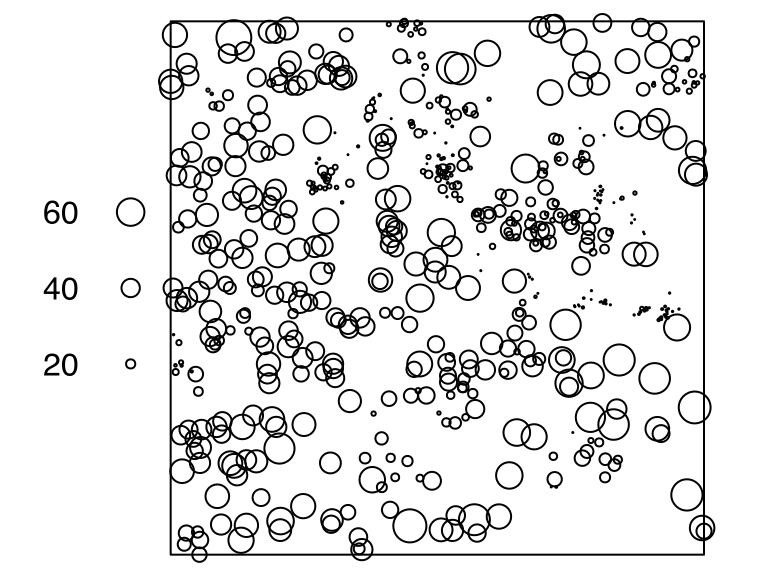
Listing 10.56: Data: longleaf

spatstat.data::longleaf |>
  spatstat.geom::print.ppp()
# Marked planar point pattern: 584 points
# marks are numeric, of storage type  'double'
# window: rectangle = [0, 200] x [0, 200] metres

10.18 `meningitis`

The spatial-object list (solist, Chapter 39) meningitis from package spatstat.data (v3.1.9, GPL (>= 2)) contains (Listing 10.58, Figure 10.12)

a point-pattern (ppp.object, Chapter 36) $cases;
a tessellation (Chapter 42) $kreise.

Listing 10.57: Figure: meningitis

Code

par(mar = c(0,0,0,0))
spatstat.data::meningitis |>
  spatstat.geom::plot.solist(main = '')

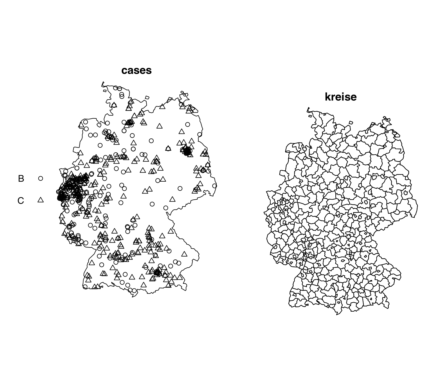
Listing 10.58: Data: meningitis

spatstat.data::meningitis
# List of spatial objects
# 
# cases:
# Marked planar point pattern: 636 points
# Multitype, with levels = B, C 
# window: polygonal boundary
# enclosing rectangle: [4031.295, 4672.253] x [2684.102, 3549.931] km
# 
# kreise:
# Tessellation
# Tiles are irregular polygons
# 413 tiles (irregular windows)
# Tessellation has a data frame of marks:
#   $marks:     double
# window: polygonal boundary
# enclosing rectangle: [4031.295, 4672.253] x [2684.102, 3549.931] km

10.19 `nbfires`

The point-pattern (ppp.object, Chapter 36) nbfires from package spatstat.data (v3.1.9, GPL (>= 2)) has (Listing 10.60, Figure 10.13)

7108 points;
polygonal window;
multi-type marks, e.g., $fire.type, $cause and $ign.src;
numeric marks, e.g., $fnl.size.

Listing 10.59: Figure: nbfires

Code

par(mar = c(0,0,1,0))
spatstat.data::nbfires |>
  spatstat.geom::plot.ppp(which.marks = c('fire.type', 'cause', 'ign.src', 'fnl.size'))
# Warning: Only 10 out of 16 symbols are shown in the symbol map

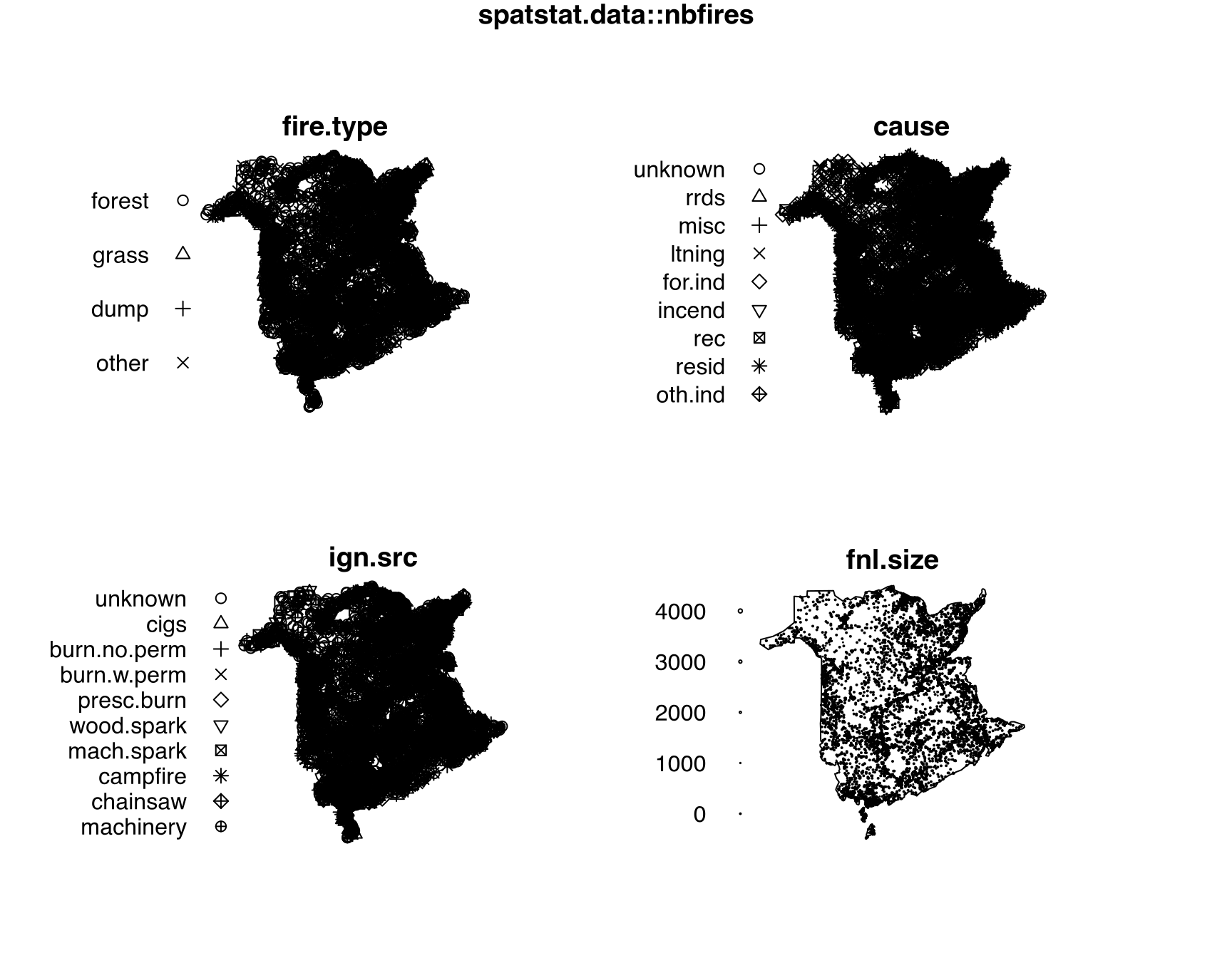
Listing 10.60: Data: nbfires

spatstat.data::nbfires |>
  spatstat.geom::print.ppp()
# Warning: some mark values are NA in the point pattern x
# Marked planar point pattern: 7108 points
# Mark variables: year, fire.type, dis.date, dis.julian, out.date, out.julian, cause, ign.src, fnl.size 
# window: polygonal boundary
# enclosing rectangle: [0, 1000] x [0, 958.9142] units (one unit = 0.403716 km)

10.20 `osteo`

The hyper data frame (hyperframe, Chapter 26) osteo from package spatstat.data (v3.1.9, GPL (>= 2)) has (Listing 10.61)

40 rows and 5 (hyper)columns (Listing 10.62)
the serial number of sampling volume $brick nested in the bone sample $id
a three-dimensional point-pattern (pp3, Chapter 35) hypercolumn $pts

Listing 10.61: Data: osteo

spatstat.data::osteo |> 
  spatstat.geom::print.hyperframe()
# Hyperframe:
#         id shortid brick   pts depth
# 1   c77za4       4     1 (pp3)    45
# 2   c77za4       4     2 (pp3)    60
# 3   c77za4       4     3 (pp3)    55
# 4   c77za4       4     4 (pp3)    60
# 5   c77za4       4     5 (pp3)    85
# ✂️ --- output truncated --- ✂️

Listing 10.62: Review: dimensions of osteo

spatstat.data::osteo |>
  spatstat.geom::dim.hyperframe()
# [1] 40  5

10.21 `spruces`

The point-pattern (ppp.object, Chapter 36) spruces from package spatstat.data (v3.1.9, GPL (>= 2)) has (Listing 10.64, Figure 10.14)

134 points;
rectangle window;
one numeric mark.

Listing 10.63: Figure: spruces

Code

par(mar = c(0,0,0,0))
spatstat.data::spruces |>
  spatstat.geom::plot.ppp(main = NULL)

Listing 10.64: Data: spruces

spatstat.data::spruces |>
  spatstat.geom::print.ppp()
# Marked planar point pattern: 134 points
# marks are numeric, of storage type  'double'
# window: rectangle = [0, 56] x [0, 38] metres

10.22 `swedishpines`

The point-pattern (ppp.object, Chapter 36) swedishpines from package spatstat.data (v3.1.9, GPL (>= 2)) has (Listing 10.66, Figure 10.15)

the $x$- and $y$-coordinates of 71 points;
rectangle window;
no marks, i.e., 'none' mark-format.

Listing 10.65: Figure: swedishpines

Code

par(mar = c(0,0,0,0))
spatstat.data::swedishpines |>
  spatstat.geom::plot.ppp(main = NULL)

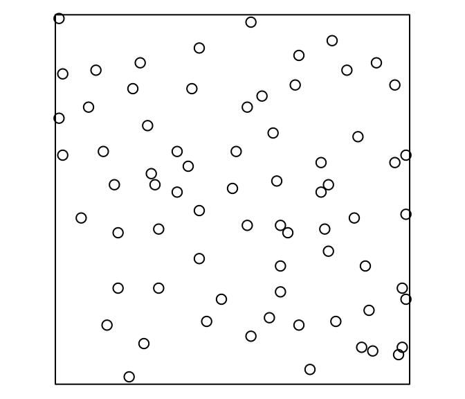
Listing 10.66: Data: swedishpines

spatstat.data::swedishpines |>
  spatstat.geom::print.ppp()
# Planar point pattern: 71 points
# window: rectangle = [0, 96] x [0, 100] units (one unit = 0.1 metres)

10.23 `VADeaths`

The matrix VADeaths from package datasets (R version 4.5.3 (2026-03-11)) has (Listing 10.67)

5 rows and 4 columns (Listing 10.68)

Listing 10.67: Data: VADeaths

datasets::VADeaths |>
  print.default()
#       Rural Male Rural Female Urban Male Urban Female
# 50-54       11.7          8.7       15.4          8.4
# 55-59       18.1         11.7       24.3         13.6
# 60-64       26.9         20.3       37.0         19.3
# 65-69       41.0         30.9       54.6         35.1
# 70-74       66.0         54.3       71.1         50.0

Listing 10.68: Review: dimensions of VADeaths

datasets::VADeaths |>
  dim()
# [1] 5 4

10.24 `vesicles`

The point-pattern (ppp.object, Chapter 36) vesicles from package spatstat.data (v3.1.9, GPL (>= 2)) has (Listing 10.70, Figure 10.16)

the $x$- and $y$-coordinates of 37 points;
polygonal window;
no marks, i.e., 'none' mark-format.

Listing 10.69: Figure: vesicles

Code

par(mar = c(0,0,0,0))
spatstat.data::vesicles |>
  spatstat.geom::plot.ppp(main = NULL)

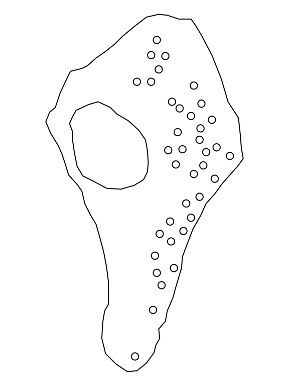
Listing 10.70: Data: vesicles

spatstat.data::vesicles |>
  spatstat.geom::print.ppp()
# Planar point pattern: 37 points
# window: polygonal boundary
# enclosing rectangle: [22.6796, 586.2292] x [11.9756, 1030.7] nm

10.25 `vesicles.extra`

The spatial-object list (solist, Chapter 39) vesicles.extra from package spatstat.data (v3.1.9, GPL (>= 2)) has (Listing 10.71, Listing 10.72)

a line-segment-pattern (psp, Chapter 38) $activezone
three windows: $mitochondria, $presynapse and $mask

Listing 10.71: Data: vesicles.extra

spatstat.data::vesicles.extra
# List of spatial objects
# 
# activezone:
# planar line segment pattern: 9 line segments
# window: rectangle = [0, 625] x [0, 1050] nm
# 
# mitochondria:
# window: polygonal boundary
# enclosing rectangle: [90.41389, 315.29187] x [532.1753, 781.4376] nm
# 
# presynapse:
# window: polygonal boundary
# enclosing rectangle: [22.6796, 586.2292] x [11.9756, 1030.7] nm
# 
# mask:
# window: binary image mask
# 420 x 250 pixel array (ny, nx)
# enclosing rectangle: [0, 250] x [0, 420] units

Listing 10.72: Review: class of members of vesicles.extra

spatstat.data::vesicles.extra |>
  lapply(FUN = class)
# $activezone
# [1] "psp"  "list"
# 
# $mitochondria
# [1] "owin"
# 
# $presynapse
# [1] "owin"
# 
# $mask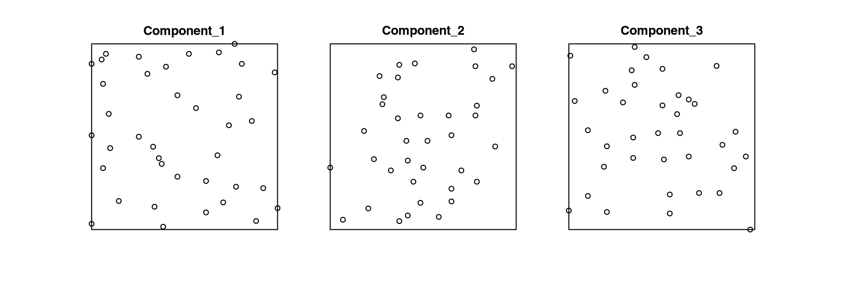
# [1] "owin"

10.26 `waterstriders`

The point-pattern-list (ppplist, Chapter 37) waterstriders from package spatstat.data (v3.1.9, GPL (>= 2)) (Listing 10.74, Figure 10.17)

inherits from the S3 class 'solist' (Chapter 39)
contains 3 point-pattern (ppp.object, Chapter 36) members (Listing 10.75).

Listing 10.73: Figure: waterstriders

Code

par(mar = c(0,0,0,0))
spatstat.data::waterstriders |> 
  spatstat.geom::plot.solist(main = '')

Listing 10.74: Data: waterstriders

spatstat.data::waterstriders
# List of point patterns
# 
# Component 1:
# Planar point pattern: 38 points
# window: rectangle = [0, 48.1] x [0, 48.1] cm
# 
# Component 2:
# Planar point pattern: 36 points
# window: rectangle = [0, 48.8] x [0, 48.8] cm
# 
# Component 3:
# Planar point pattern: 36 points
# window: rectangle = [0, 46.4] x [0, 46.4] cm

Listing 10.75: Review: class of members of waterstriders

spatstat.data::waterstriders |> 
  sapply(FUN = class)
# [1] "ppp" "ppp" "ppp"

10.1 anemones

10.2 ants

10.3 austates

10.4 betacells

10.5 bronzefilter

10.6 btb.extra

10.7 cars

10.8 cetaceans

10.9 demohyper

10.10 faithful

10.11 finpines

10.12 flu

10.13 gorillas

10.14 gorillas.extra

10.15 hyytiala

10.16 Kovesi

10.17 longleaf

10.18 meningitis

10.19 nbfires

10.20 osteo

10.21 spruces

10.22 swedishpines

10.23 VADeaths

10.24 vesicles

10.25 vesicles.extra

10.26 waterstriders

10.1 `anemones`

10.2 `ants`

10.3 `austates`

10.4 `betacells`

10.5 `bronzefilter`

10.6 `btb.extra`

10.7 `cars`

10.8 `cetaceans`

10.9 `demohyper`

10.10 `faithful`

10.11 `finpines`

10.12 `flu`

10.13 `gorillas`

10.14 `gorillas.extra`

10.15 `hyytiala`

10.16 `Kovesi`

10.17 `longleaf`

10.18 `meningitis`

10.19 `nbfires`

10.20 `osteo`

10.21 `spruces`

10.22 `swedishpines`

10.23 `VADeaths`

10.24 `vesicles`

10.25 `vesicles.extra`

10.26 `waterstriders`