20  fv

ImportantDisclaimer

These packages (Note 1) are a one-person project undergoing rapid evolution. Backward compatibility (per Hadley Wickham) is provided as a courtesy rather than a guarantee.

Until further notice, these packages should

  • not be used as a basis for research grant applications,
  • not be cited as an actively maintained tool in a peer-reviewed manuscript,
  • not be used to support or fulfill requirements for pursuing an academic degree.

In addition, work primarily based on these packages (Note 1) should not be presented at academic conferences or similar scholarly venues.

Furthermore, a person’s ability to use these packages (Note 1) does not necessarily imply an understanding of their underlying mechanisms. Accordingly, demonstration of their use alone should not be considered sufficient evidence of expertise, nor should it be credited as a basis for academic promotion or advancement.

These statements do not apply to the contributors (Tip 1) to these packages (Note 1) with respect to their specific contributions.

These statements do not apply when the maintainer of these packages (Note 1), Tingting Zhan, is credited as the first author, the lead author, and/or the corresponding author in a peer-reviewed manuscript, or as the Principal Investigator or Co-Principal Investigator in a research grant application and/or a final research progress report.

These statements are advisory in nature and do not modify or restrict the rights granted under the GNU General Public License https://www.r-project.org/Licenses/.

The function fv() (v3.8.0, GPL (>= 2)) creates a function-value-table (fv.object), i.e., an R object of S3 class 'fv'.

The S3 generic function as.fv() (v3.8.0, GPL (>= 2)) converts R objects of various classes into a function-value-table. Listing 20.1 summarizes the S3 methods for the generic function as.fv() in the spatstat.* family of packages,

Listing 20.1: S3 methods spatstat.*::as.fv.*
Code
library(spatstat)
.S3methods(generic.function = 'as.fv', all.names = TRUE) |> 
  attr(which = 'info', exact = TRUE) |>
  subset.data.frame(subset = grepl(pattern = '^spatstat\\.', x = from))
#                  visible             from generic  isS4
# as.fv.bw.optim      TRUE spatstat.explore   as.fv FALSE
# as.fv.data.frame    TRUE spatstat.explore   as.fv FALSE
# as.fv.dppm          TRUE   spatstat.model   as.fv FALSE
# as.fv.fasp          TRUE spatstat.explore   as.fv FALSE
# as.fv.fv            TRUE spatstat.explore   as.fv FALSE
# as.fv.kppm          TRUE   spatstat.model   as.fv FALSE
# as.fv.matrix        TRUE spatstat.explore   as.fv FALSE
# as.fv.minconfit     TRUE   spatstat.model   as.fv FALSE

Listing 20.2 summarizes the S3 methods for the class 'fv' in the spatstat.* family of packages,

Listing 20.2: S3 methods spatstat.*::*.fv
Code
library(spatstat)
.S3methods(class = 'fv', all.names = TRUE) |> 
  attr(which = 'info', exact = TRUE) |>
  subset.data.frame(subset = grepl(pattern = '^spatstat\\.', x = from))
#                  visible             from       generic  isS4
# [.fv                TRUE spatstat.explore             [ FALSE
# [<-.fv              TRUE spatstat.explore           [<- FALSE
# $<-.fv              TRUE spatstat.explore           $<- FALSE
# as.data.frame.fv    TRUE spatstat.explore as.data.frame FALSE
# as.function.fv      TRUE spatstat.explore   as.function FALSE
# as.fv.fv            TRUE spatstat.explore         as.fv FALSE
# cbind.fv            TRUE spatstat.explore         cbind FALSE
# collapse.fv         TRUE spatstat.explore      collapse FALSE
# compatible.fv       TRUE spatstat.explore    compatible FALSE
# Complex.fv          TRUE spatstat.explore       Complex FALSE
# deriv.fv            TRUE spatstat.explore         deriv FALSE
# formula.fv          TRUE spatstat.explore       formula FALSE
# formula<-.fv        TRUE spatstat.explore     formula<- FALSE
# harmonise.fv        TRUE spatstat.explore     harmonise FALSE
# harmonize.fv        TRUE spatstat.explore     harmonize FALSE
# integral.fv         TRUE spatstat.explore      integral FALSE
# Math.fv             TRUE spatstat.explore          Math FALSE
# names<-.fv          TRUE spatstat.explore       names<- FALSE
# Ops.fv              TRUE spatstat.explore           Ops FALSE
# pcf.fv              TRUE spatstat.explore           pcf FALSE
# plot.fv             TRUE spatstat.explore          plot FALSE
# pool.fv             TRUE spatstat.explore          pool FALSE
# print.fv            TRUE spatstat.explore         print FALSE
# rose.fv             TRUE spatstat.explore          rose FALSE
# Smooth.fv           TRUE spatstat.explore        Smooth FALSE
# StieltjesCalc.fv    TRUE spatstat.explore StieltjesCalc FALSE
# Summary.fv          TRUE spatstat.explore       Summary FALSE
# with.fv             TRUE spatstat.explore          with FALSE
Note

The examples in Chapter 20 require

library(groupedHyperframe)

Table 20.1 summarizes the S3 methods for the class 'fv' in package groupedHyperframe (v0.4.0, GPL-2),

Table 20.1: S3 methods groupedHyperframe::*.fv (v0.4.0)
visible generic isS4
.disrecommend2theo.fv FALSE groupedHyperframe::.disrecommend2theo FALSE
.illegal2theo.fv FALSE groupedHyperframe::.illegal2theo FALSE
.rmax.fv FALSE groupedHyperframe::.rmax FALSE
cumvtrapz.fv FALSE groupedHyperframe::cumvtrapz FALSE
keyval.fv FALSE groupedHyperframe::keyval FALSE
visualize_vtrapz.fv FALSE groupedHyperframe::visualize_vtrapz FALSE

20.1 Example

Listing 20.3 creates a function-value-table spruces_k, which is the mark correlation of the point-pattern spruces (Section 10.21).

Listing 20.3: Data: function-value-table spruces_k
spruces_k = spatstat.data::spruces |> 
  spatstat.explore::markcorr()

The S3 method print.fv() (v3.8.0, GPL (>= 2)) (Listing 20.4) prints the vital information of a function-value-table.

Listing 20.4: Review: function print.fv() (Listing 20.3)
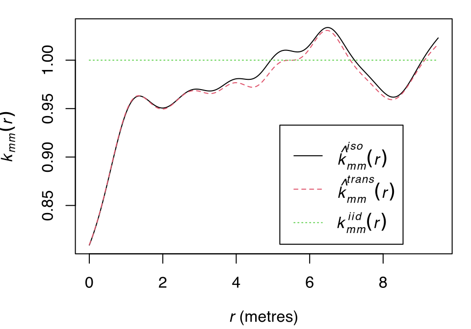
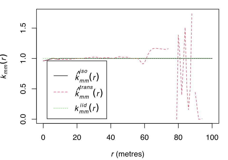
spruces_k |>
  spatstat.explore::print.fv()
# Function value object (class 'fv')
# for the function r -> k[mm](r)
# ................................................................................
#       Math.label              Description                                       
# r     r                       distance argument r                               
# theo  {k[mm]^{iid}}(r)        theoretical value (independent marks) for k[mm](r)
# trans {hat(k)[mm]^{trans}}(r) translation-corrected estimate of k[mm](r)        
# iso   {hat(k)[mm]^{iso}}(r)   Ripley isotropic correction estimate of k[mm](r)  
# ................................................................................
# Default plot formula:  .~r
# where "." stands for 'iso', 'trans', 'theo'
# Recommended range of argument r: [0, 9.5]
# Available range of argument r: [0, 9.5]
# Unit of length: 1 metre

The S3 method plot.fv() (v3.8.0, GPL (>= 2)) (Listing 20.5) visualizes the recommended function values of spruces_k (Listing 20.3) as a black-solid-curve (Figure 20.1).

Listing 20.5: Review: function plot.fv() (Listing 20.3)
par(mar = c(4, 4, 1, 1))
spruces_k |>
  spatstat.explore::plot.fv(main = NULL)
Figure 20.1: Mark Correlation of spruces (Listing 20.3)

The function fvnames() (v3.8.0, GPL (>= 2)) finds the columns in a function-value-table that are (Table 20.2, Listing 20.6),

Table 20.2: Function fvnames()
Abbreviation Finds
a = '.x' the function argument
a = '.y' the recommended function value
Listing 20.6: Review: function fvnames() (Listing 20.3)
c(
  .x = spruces_k |>
    spatstat.explore::fvnames(a = '.x'),
  .y = spruces_k |>
    spatstat.explore::fvnames(a = '.y')
)
#    .x    .y 
#   "r" "iso"

20.2 Function Value

The S3 generic function keyval(), for key value, finds various function values (default being the recommended) in a function-value-table, or an R object containing one or more function-value-tables. The term “key” comes from the invisible return of the S3 method plot.fv() (v3.8.0, GPL (>= 2)) (Listing 20.7). Package groupedHyperframe (v0.4.0, GPL-2) implements the following S3 methods (Table 20.3),

Table 20.3: S3 methods of groupedHyperframe::keyval (v0.4.0)
visible generic isS4
keyval.fv FALSE groupedHyperframe::keyval FALSE
Listing 20.7: Review: the invisible return of function plot.fv()
noprt = spatstat.explore::plot.fv |>
  body() |>
  tail(n = 2L) |>
  lapply(FUN = print.default)
# df <- data.frame(lty = lty, col = col, key = key, label = labl, 
#     meaning = legdesc, row.names = key)
# return(invisible(df))

The S3 method keyval.fv() finds various function values (default being the recommended) in a function-value-table, with the corresponding function argument as the vector names.

Listing 20.8 finds the recommended function value in the function-value-table spruces_k (Listing 20.3).

Listing 20.8: Example: function keyval.fv() (Listing 20.3)
spruces_k_iso = spruces_k |>
  keyval()
spruces_k_iso
#            0 0.0185546875  0.037109375 0.0556640625   0.07421875 0.0927734375  0.111328125 0.1298828125    0.1484375 0.1669921875  0.185546875 0.2041015625   0.22265625 0.2412109375  0.259765625 
#    0.8091085    0.8109143    0.8128058    0.8147079    0.8166921    0.8186921    0.8207701    0.8228690    0.8250411    0.8272393    0.8295051    0.8318018    0.8341601    0.8365537    0.8390019 
# ✂️ --- output truncated --- ✂️

Listing 20.9 finds the theoretical function value in the function-value-table spruces_k (Listing 20.3).

Listing 20.9: Example: function keyval.fv(., key = 'theo') (Listing 20.3)
spruces_k_theo = spruces_k |>
  keyval(key = 'theo')
spruces_k_theo
#            0 0.0185546875  0.037109375 0.0556640625   0.07421875 0.0927734375  0.111328125 0.1298828125    0.1484375 0.1669921875  0.185546875 0.2041015625   0.22265625 0.2412109375  0.259765625 
#            1            1            1            1            1            1            1            1            1            1            1            1            1            1            1 
# ✂️ --- output truncated --- ✂️

The S3 method with.fv() (v3.8.0, GPL (>= 2)) is capable of creating identical returns as the S3 method keyval.fv() (Listing 20.10, Listing 20.11). The internal utility function getValues() defined in the local environment of the S3 group-generic-method Summary.fv() (Listing 20.12) vectorizes all function values. Table 20.4 explains their differences and connections.

Listing 20.10: Review: function with.fv(), identical to Listing 20.8
spruces_k |>
  spatstat.explore::with.fv(expr = setNames(iso, nm = r)) |>
  identical(y = spruces_k_iso) |> 
  stopifnot()
Listing 20.11: Review: function with.fv(), identical to Listing 20.9
spruces_k |>
  spatstat.explore::with.fv(expr = setNames(theo, nm = r)) |>
  identical(y = spruces_k_theo) |> 
  stopifnot()
Listing 20.12: Review: function getValues() defined in the local environment of function Summary.fv()
spatstat.explore::Summary.fv |>
  environment() |>
  get(x = 'getValues', envir = _)
# function (x) 
# {
#     xdat <- as.matrix(as.data.frame(x))
#     yall <- fvnames(x, ".")
#     vals <- xdat[, yall]
#     return(as.vector(vals))
# }
# <environment: 0x13c645e50>
Table 20.4: Functions keyval.fv(), etc.
keyval.fv() with.fv() getValues()
Finds Specific function value Very flexible All function values
Speed Fast Slow Fast
Closure Namespace of package groupedHyperframe (v0.4.0, GPL-2) Namespace of package spatstat.explore (v3.8.0, GPL (>= 2)) Local environment of Summary.fv()

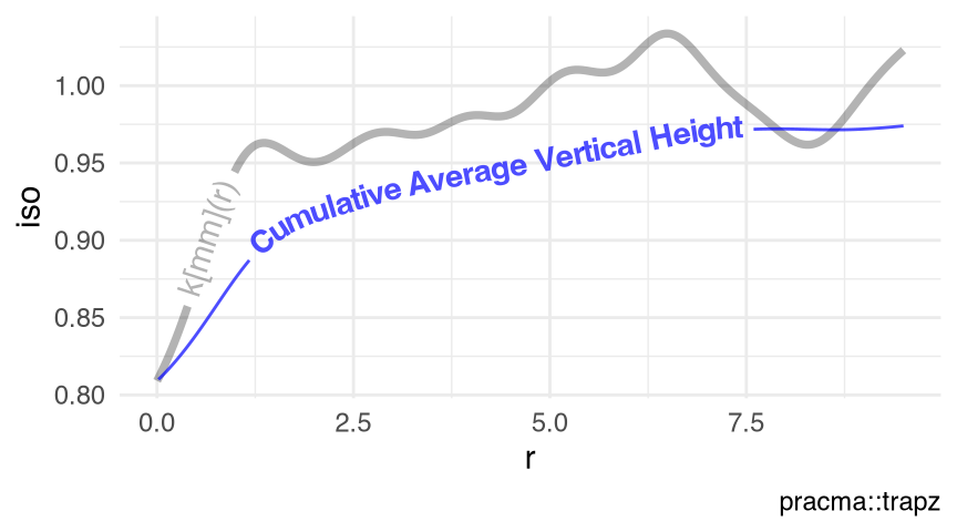
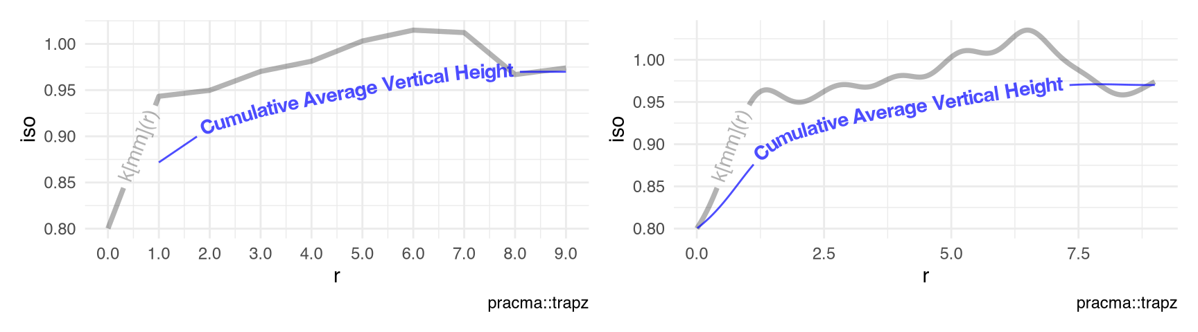
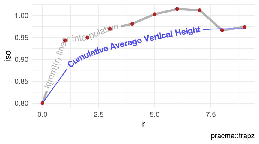
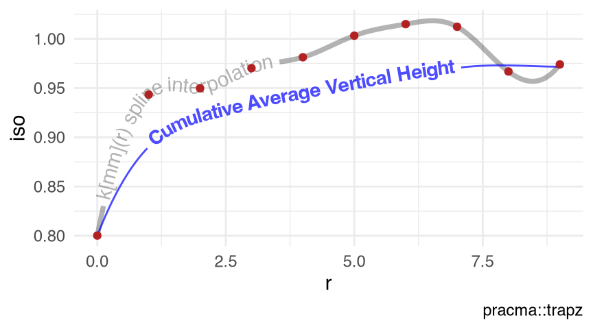
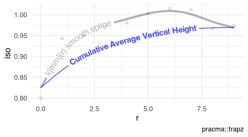
20.3 Cumulative Average Vertical Height of Trapzoidal Integration

The S3 method cumvtrapz.fv() (Section 11.2, Table 11.1) calculates the cumulative average vertical height of the trapezoidal integration (Section 11.2) under the recommended function values.

The S3 method visualize_vtrapz.fv() (Section 11.3, Table 11.2) visualizes the cumulative average vertical height of the trapezoidal integration (Section 11.2) under the recommended function values

Listing 20.13 finds the cumulative average vertical height of the trapezoidal integration of the function-value-table spruces_k (Listing 20.3). Listing 20.14 visualizes Listing 20.13 in Figure 20.2.

Listing 20.13: Example: function cumvtrapz.fv() (Listing 20.3)
spruces_k |>
  cumvtrapz()
#             [,1]
#   [1,] 0.8100114
#   [2,] 0.8109357
#   [3,] 0.8118761
# ✂️ --- output truncated --- ✂️
Listing 20.14: Figure: function visualize_vtrapz.fv() (Listing 20.3)
spruces_k |>
  visualize_vtrapz(draw.rect = FALSE)
Figure 20.2: Cumulative Average Vertical Height of the Trapezoidal Integration (Section 11.2) of spruces_k (Listing 20.3)

20.4 \(r_\text{max}\)

The S3 method .rmax.fv() (Section 36.9, Table 36.13), often used as an internal utility function, simply grabs the maximum value of the \(r\)-vector in a function-value-table.

Listing 20.15 finds the maximum value of the \(r\)-vector in the function-value-table spruces_k (Listing 20.3). Listing 20.16 creates an identical return as Listing 20.15 using the S3 method with.fv() (v3.8.0, GPL (>= 2)).

Listing 20.15: Example: function .rmax.fv() (Listing 20.3)
sprucesK_r = spruces_k |>
  .rmax()
sprucesK_r
# [1] 9.5
Listing 20.16: Review: function with.fv(), identical to Listing 20.15
spruces_k |>
  spatstat.explore::with.fv(expr = max(r)) |>
  identical(y = sprucesK_r) |> 
  stopifnot()

20.5 Legal \(r_\text{max}\)

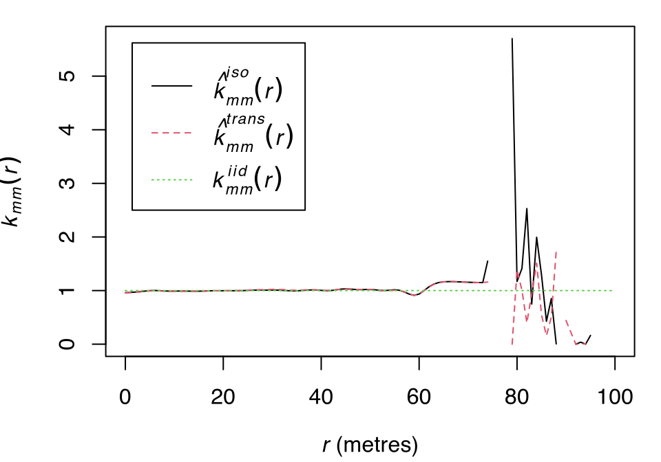
The function markcorr() (v3.8.0, GPL (>= 2)) is the workhorse inside the functions Emark(), Vmark() and markvario() (v3.8.0, GPL (>= 2)). Function markcorr() provides a default argument of parameter \(r\)-vector (Section 36.9), at which the mark correlation function \(k_f(r)\) are evaluated. Function markcorr() relies on the un-exported workhorse function spatstat.explore:::sewsmod(), whose default method = "density" contains a ratio of two kernel density estimates. Exceptional/illegal values of 0, Inf and/or NaN (Chapter 47, Listing 47.1) may appear in the return of function markcorr(), if the \(r\)-vector goes well beyond the recommended range (Listing 20.4).

Listing 20.17 constructs a malformed function-value-table fv_mal (Figure 20.3).

Listing 20.17: Data: a malformed function-value-table fv_mal with \(r\)-vector out-of-range
fv_mal = spatstat.data::spruces |> 
  spatstat.explore::markcorr(r = 0:100)
Listing 20.18: Review: plot.fv() on fv_mal (Listing 20.17)
Code
par(mar = c(4, 4, 1, 1))
fv_mal |> 
  spatstat.explore::plot.fv(xlim = c(0, 100), main = NULL)
Figure 20.3: A malformed function-value-table fv_mal (Listing 20.17)

The term Legal \(r_\text{max}\) indicates (the index) of the \(r\)-vector, where the last of the consecutive legal (Chapter 47, Listing 47.5) recommended function values appears. Listing 20.19 shows that the last consecutive legal recommended-function-value of the malformed function-value-table fv_mal (Listing 20.17) of \(k_f(r)=1.550\) appears at the 75-th index of the \(r\)-vector, i.e., \(r=74\).

Listing 20.19: Example: lastLegal() of keyval.fv() (Listing 20.17)
spruces_k_lastLegal = fv_mal |>
  keyval() |>
  lastLegal()
spruces_k_lastLegal
# [1] 75
# attr(,"value")
#       74 
# 1.549766

Legality of the function markcorr() returns depends not only on the input point-pattern, but also on the values of the \(r\)-vector (Listing 20.20). In other words, the creation of a function-value-table is a numerical procedure. Therefore, the discussion of Legal \(r_\text{max}\) pertains to the function-value-table (fv.object, Chapter 20), instead of to the point-pattern (ppp.object, Chapter 36).

Listing 20.20: Example: Legality of markcorr() return depends on \(r\)-vector
spatstat.data::spruces |> 
  spatstat.explore::markcorr(r = seq.int(from = 0, to = 100, by = .1)) |>
  keyval() |>
  lastLegal()
# [1] 742
# attr(,"value")
#      74.1 
# 0.3191326

20.5.1 Handling Illegal Recommended-Function-Value

The S3 generic functions .illegal2theo() and .disrecommend2theo() are exploratory approaches to remove the illegal recommended function values (Section 20.5) from a function-value-table. These approaches replace the recommended function values with the theoretical values starting at different locations in the function argument (Table 20.2, Listing 20.6), and return an updated function-value-table. Package groupedHyperframe (v0.4.0, GPL-2) implements the following S3 methods (Table 20.5, Table 20.6),

Table 20.5: S3 methods of groupedHyperframe::.illegal2theo (v0.4.0)
visible generic isS4
.illegal2theo.fv FALSE groupedHyperframe::.illegal2theo FALSE
Table 20.6: S3 methods of groupedHyperframe::.disrecommend2theo (v0.4.0)
visible generic isS4
.disrecommend2theo.fv FALSE groupedHyperframe::.disrecommend2theo FALSE

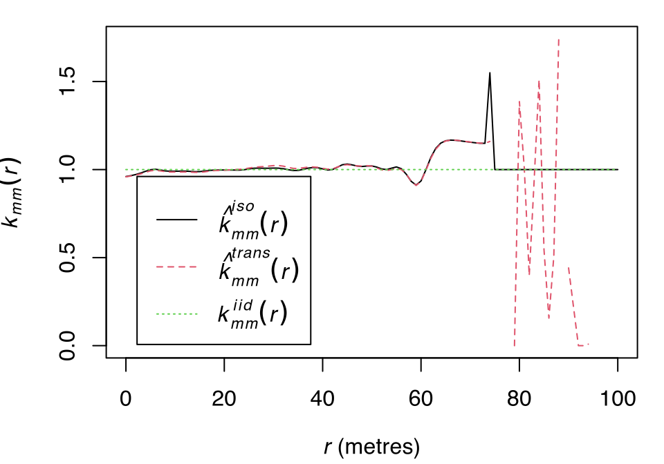
The S3 method .illegal2theo.fv() (Listing 20.21) replaces the recommended function values after the first illegal \(r\) (Section 20.5) of the malformed function-value-table fv_mal (Listing 20.17) with its theoretical values (Figure 20.4).

Listing 20.21: Advanced: function .illegal2theo.fv() (Listing 20.17)
par(mar = c(4, 4, 1, 1))
fv_mal |> 
  .illegal2theo() |>
  spatstat.explore::plot.fv(xlim = c(0, 100), main = NULL)
# r≥75.0 replaced with theo
Figure 20.4: Replaces with theoretical values after the first illegal \(r\) (Listing 20.17)

The S3 method .disrecommend2theo.fv() (Listing 20.22) replaces the recommended function values outside the recommended range attr(.,'alim')[2L] of the malformed function-value-table fv_mal (Listing 20.17) with its theoretical values (Figure 20.5).

Listing 20.22: Advanced: function .disrecommend2theo.fv() (Listing 20.17)
par(mar = c(4, 4, 1, 1))
fv_mal |> 
  .disrecommend2theo() |>
  spatstat.explore::plot.fv(xlim = c(0, 100), main = NULL)
# r≥10.0 replaced with theo
Figure 20.5: Replaces with theoretical values outside the recommended range (Listing 20.17)

20.6 Interpolation & Smoothing

This section illustrates various interpolation (Section 20.6.1) and smoothing methods (Section 20.6.2) of the \(x\)- and \(y\)-values (Table 20.2, Listing 20.6) in a function-value-table.

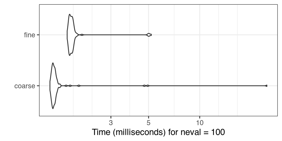
Listing 20.23 creates the toy examples of a coarse and a fine function-value-table at a coarse and a fine \(r\)-vector for the mark correlation of the point-pattern spruces (Section 10.21).

Listing 20.23: Data: coarse versus fine function-value-table
r = list(
  coarse = 0:9,
  fine = seq.int(from = 0, to = 9, by = .01)
)
sprucesK = r |> 
  lapply(FUN = \(r) {
    spatstat.data::spruces |>
      spatstat.explore::markcorr(r = r)
  })
Listing 20.24: Figure: coarse versus fine function-value-table, trapezoidal integration (Listing 20.23)
sprucesK |>
  groupedHyperframe:::visualize_vtrapz.listof(draw.rect = FALSE)
Figure 20.6: coarse versus fine function-value-table, trapezoidal integration (Listing 20.23)

20.6.1 Interpolation

20.6.1.1 Linear Interpolation

The function approxfun.fv() creates a linear interpolation from a function-value-table and returns an R object of S3 class 'function'. This is a “pseudo” S3 method, as the workhorse function approxfun() is not an S3 generic function.

Listing 20.25 creates a linear interpolation (Figure 20.7) of the coarse function-value-table sprucesK$coarse (Listing 20.23), which is mathematically equivalent to the return of the S3 method as.function.fv() (v3.8.0, GPL (>= 2)) (Listing 20.26).

Listing 20.25: Example: function approxfun.fv() (Listing 20.23)
sprucesK$coarse |> 
  approxfun.fv() |>
  visualize_vtrapz(draw.rect = FALSE)
Figure 20.7: Linear Interpolation approxfun.fv()
Listing 20.26: Review: function approxfun.fv() equivalent to as.function.fv() (Listing 20.23)
Code
sprucesK$coarse |> 
  approxfun.fv() |>
  do.call(what = _, args = list(v = r$coarse)) |>
  identical(
    y = sprucesK$coarse |>  
      spatstat.explore::as.function.fv() |>
      do.call(what = _, args = list(r = r$coarse))
  ) |>
  stopifnot()

20.6.1.2 Spline Interpolation

The function splinefun.fv() creates a spline interpolation from a function-value-table and returns an R object of S3 class 'function'. This is a “pseudo” S3 method, as the workhorse function splinefun() is not an S3 generic function.

Listing 20.27 creates a spline interpolation (Figure 20.8) of the coarse function-value-table sprucesK$coarse (Listing 20.23).

Listing 20.27: Example: function splinefun.fv() (Listing 20.23)
sprucesK$coarse |> 
  splinefun.fv() |>
  visualize_vtrapz(draw.rect = FALSE)
Figure 20.8: Spline Interpolation splinefun.fv()

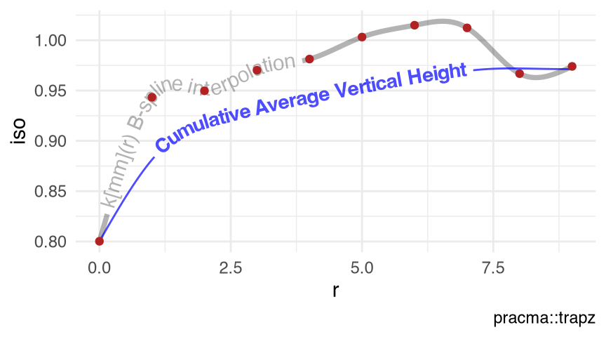
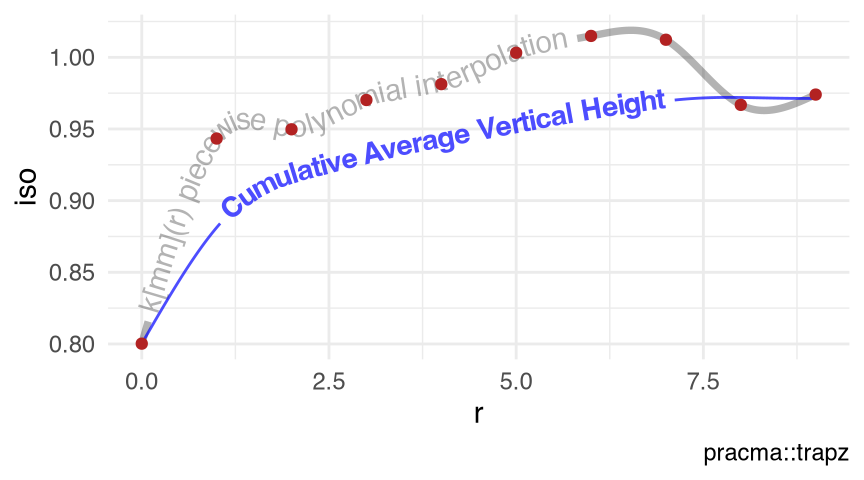
The function interpSpline_.fv() creates a B-spline or a piecewise polynomial spline interpolation from a function-value-table and returns an R object of S3 class 'spline'. This is a “pseudo” S3 method, as the parameterization of the workhorse S3 generic function splines::interpSpline() is not ideal for this purpose.

Listing 20.28 creates a B-spline interpolation (Figure 20.9) of the coarse function-value-table sprucesK$coarse (Listing 20.23).

Listing 20.28: Example: function interpSpline_.fv(., bSpline = TRUE) (Listing 20.23)
sprucesK$coarse |> 
  interpSpline_.fv(bSpline = TRUE) |>
  visualize_vtrapz(draw.rect = FALSE)
Figure 20.9: B-Spline Interpolation interpSpline_.fv(., bSpline = TRUE)

Listing 20.29 creates a piecewise polynomial interpolation (Figure 20.10) of the coarse function-value-table sprucesK$coarse (Listing 20.23).

Listing 20.29: Example: function interpSpline_.fv() (Listing 20.23)
sprucesK$coarse |> 
  interpSpline_.fv() |>
  visualize_vtrapz(draw.rect = FALSE)
Figure 20.10: Piecewise Polynomial Spline Interpolation interpSpline_.fv()

20.6.2 Smoothing

20.6.2.1 Local Polynomial Regression

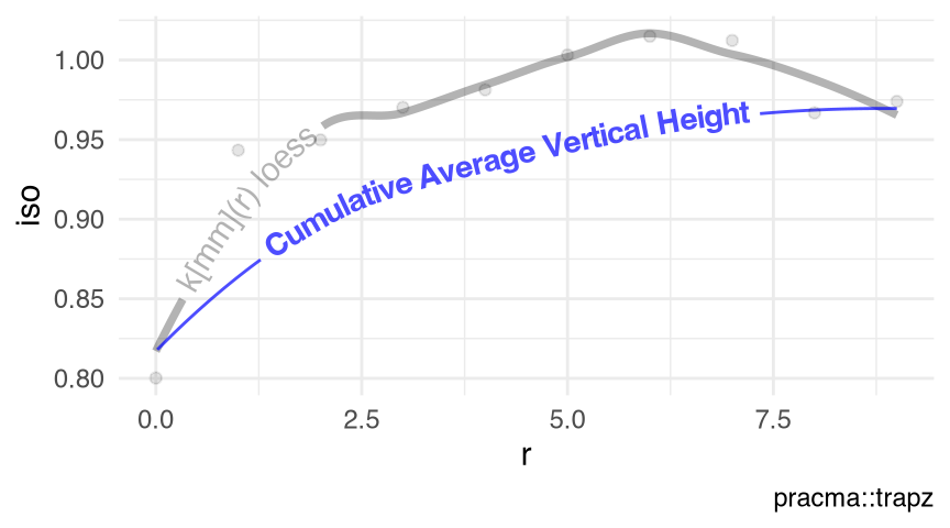
The function loess.fv() creates a local polynomial regression fit from a function-value-table and returns an R object of S3 class 'loess'. This is a “pseudo” S3 method, as the workhorse function loess() is not an S3 generic function.

Listing 20.30 creates a local polynomial regression (Figure 20.11) of the coarse function-value-table sprucesK$coarse (Listing 20.23), which is mathematically equivalent to the return of the S3 method Smooth.fv() (v3.8.0, GPL (>= 2)) with 'loess' method (Listing 20.31).

Listing 20.30: Example: function loess.fv() (Listing 20.23)
sprucesK$coarse |> 
  loess.fv() |>
  visualize_vtrapz(draw.rect = FALSE)
Figure 20.11: Local Polynomial Regression, or LOESS, loess.fv()
Listing 20.31: Review: predicted values of function loess.fv() equivalent to Smooth.fv(., method = 'loess') (Listing 20.23)
Code
sprucesK$coarse |> 
  loess.fv() |> 
  stats:::predict.loess(newdata = r$coarse) |> 
  identical(
    y = sprucesK$coarse |>
      spatstat.explore::Smooth.fv(method = 'loess') |>
      spatstat.explore::with.fv(expr = iso)
  ) |>
  stopifnot()

20.6.2.2 Kernel Regression Smoother

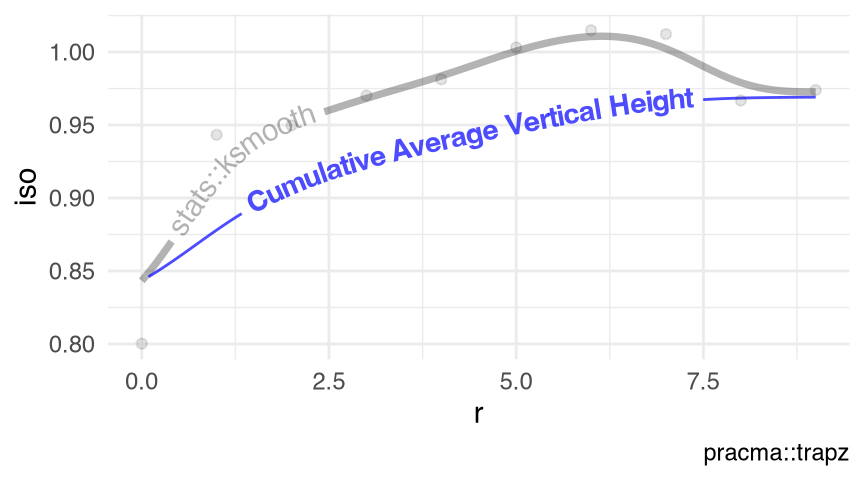
The function ksmooth.fv() creates a kernel regression smoother from a function-value-table and returns an R object of S3 class 'ksmooth'. This is a “pseudo” S3 method, as the workhorse function ksmooth() is not an S3 generic function.

Listing 20.32 creates a kernel regression smoother (Figure 20.12) of the coarse function-value-table sprucesK$coarse (Listing 20.23).

Listing 20.32: Example: function ksmooth.fv() (Listing 20.23)
sprucesK$coarse |> 
  ksmooth.fv(kernel = 'normal', bandwidth = 2) |>
  visualize_vtrapz(draw.rect = FALSE)
Figure 20.12: kernel regression smoother ksmooth.fv()

20.6.2.3 Smoothing Spline

The function smooth.spline.fv() creates a smoothing spline from a function-value-table and returns an R object of S3 class 'smooth.spline'. This is a “pseudo” S3 method, as the workhorse function smooth.spline() is not an S3 generic function.

Listing 20.33 creates a smoothing spline (Figure 20.13) of the coarse function-value-table sprucesK$coarse (Listing 20.23), which is mathematically equivalent to the return of the S3 method Smooth.fv() (v3.8.0, GPL (>= 2)) with 'smooth.spline' method (Listing 20.34).

Listing 20.33: Example: function smooth.spline.fv() (Listing 20.23)
sprucesK$coarse |> 
  smooth.spline.fv(df = 5L) |>
  visualize_vtrapz(draw.rect = FALSE)
Figure 20.13: Smoothing Spline smooth.spline.fv()
Listing 20.34: Review: predicted values of function smooth.spline.fv() equivalent to Smooth.fv(., method = 'smooth.spline') (Listing 20.23)
Code
sprucesK$coarse |> 
  smooth.spline.fv(df = 5L) |> 
  stats:::predict.smooth.spline(x = r$coarse) |> 
  with.default(expr = y) |> 
  identical(
    y = sprucesK$coarse |>
      spatstat.explore::Smooth.fv(method = 'smooth.spline', df = 5L) |>
      spatstat.explore::with.fv(expr = iso)
  ) |>
  stopifnot()

20.6.3 Benchmarks

An experienced reader may wonder: is it truly advantageous to compute a coarse function-value-table sprucesK$coarse and then perform interpolation (Section 20.6.1) and/or smoothing (Section 20.6.2), rather than computing a fine function-value-table sprucesK$fine to start with? This is an excellent question! As of package spatstat.explore (v3.8.0, GPL (>= 2)), we observe only minor increase in the computation time of the creation of a function-value-table, even when the grid of the \(r\)-vector is 100 times finer (Listing 20.35, Figure 20.14) via package microbenchmark (Mersmann 2024, v1.5.0, BSD_2_clause + file LICENSE). This observation justifies the use of the plain-and-naïve trapezoidal integration (Chapter 11, Section 11.2) on a fine function-value-table (Figure 20.6, Right), rather than employing more sophisticated numerical integration methods, e.g.,

on an interpolation and/or smoothing of a coarse function-value-table.

Listing 20.35: Benchmark: coarse versus fine function-value-table (Listing 20.23)
library(spatstat)
microbenchmark::microbenchmark(
  coarse = markcorr(spruces, r = r$coarse),
  fine = markcorr(spruces, r = r$fine)
) |>
  microbenchmark:::autoplot.microbenchmark() +
  ggplot2::labs(title = NULL) +
  ggplot2::theme_bw()
Figure 20.14: Benchmarks (Mersmann 2024): coarse versus fine function-value-table