11 Trapezoidal Integration

Disclaimer

These packages (Note 1) are a one-person project undergoing rapid evolution. Backward compatibility (per Hadley Wickham) is provided as a courtesy rather than a guarantee.

Until further notice, these packages should

not be used as a basis for research grant applications,
not be cited as an actively maintained tool in a peer-reviewed manuscript,
not be used to support or fulfill requirements for pursuing an academic degree.

In addition, work primarily based on these packages (Note 1) should not be presented at academic conferences or similar scholarly venues.

Furthermore, a person’s ability to use these packages (Note 1) does not necessarily imply an understanding of their underlying mechanisms. Accordingly, demonstration of their use alone should not be considered sufficient evidence of expertise, nor should it be credited as a basis for academic promotion or advancement.

These statements do not apply to the contributors (Tip 1) to these packages (Note 1) with respect to their specific contributions.

These statements do not apply when the maintainer of these packages (Note 1), Tingting Zhan, is credited as the first author, the lead author, and/or the corresponding author in a peer-reviewed manuscript, or as the Principal Investigator or Co-Principal Investigator in a research grant application and/or a final research progress report.

These statements are advisory in nature and do not modify or restrict the rights granted under the GNU General Public License https://www.r-project.org/Licenses/.

Examples in Chapter 11 Require

library(groupedHyperframe)

11.1 Chained Trapezoidal Rule

The chained trapezoidal rule of numerically approximating a definite integral is an ancient idea since the dawn of human civilization.

Let $\{x_k; k=0,\cdots,N\}$ be a partition of the real interval $[a,b]$ such that $a = x_0 < x_1 < \cdots < x_{N-1} < x_N = b$ and $\Delta x_k= x_k - x_{k-1}$ be the length of the $k$-th sub-interval, then the chained-trapezoidal approximation of the integration of the function $y=f(x)$ is,

\[ \begin{split} \int_a^b f(x)\,dx & \approx \sum_{k=1}^{N}{\dfrac{y_{k-1}+y_k}{2}}\Delta x_{k} \\ & = \left(\frac{y_0}{2}+\sum _{k=1}^{N-1}y_k+\frac{y_N}{2}\right)\Delta x, \quad\iff\ \forall k, \Delta x_{k}\equiv \Delta x \end{split} \tag{11.1}\]

Listing 11.1 creates a toy example of two numeric vectors x $=(x_0,x_1,x_2,x_3,x_4,x_5)^t$ and y $=\{y_k = f(x_k);k=0,1,\cdots,5\}$. The numeric vector x is intentionally made non-equidistant, as neither the chained trapezoidal rule framework nor the functions trapz() and cumtrapz() (Borchers 2025, v2.4.6, GPL (>= 3)) requires the equidistant assumption.

Listing 11.1: Data: toy example x and y

x. = seq.int(from = 10L, to = 20L, by = 2L)
set.seed(23); x = rnorm(n = length(x.), mean = x., sd = .5)
set.seed(12); y = rnorm(n = length(x.), mean = 1, sd = .3)
list(x = x, y = y)
# $x
# [1] 10.09661 11.78266 14.45663 16.89669 18.49830 20.55375
# 
# $y
# [1] 0.5558297 1.4731508 0.7129767 0.7239984 0.4007074 0.9183112

Listing 11.2 calculates the trapezoidal integration (Equation 11.1, Figure 11.1) of the toy example x and y (Listing 11.1).

Listing 11.2: Review: function trapz() (Listing 11.1)

pracma::trapz(x, y)
# [1] 8.642715

In R nomenclature, the term “cumulative” indicates an inclusive scan, in other words,

Inclusive Scan

The ith element of the output is the operation result of the first-i-elements of the input.

For example, Listing 11.3 is a summation, while Listing 11.4 is a cumulative summation.

Listing 11.3: Review: function sum()

sum(1:5)
# [1] 15

Listing 11.4: Review: function cumsum()

cumsum(1:5)
# [1]  1  3  6 10 15

Listing 11.5 calculates the cumulative trapezoidal integration of the toy example x and y (Listing 11.1). Note that the first element of the output is always 0, as a trapezoidal integration needs at least two points of $\left(x_0, y_0\right)$ and $\left(x_1, y_1\right)$.

Listing 11.5: Review: function cumtrapz() (Listing 11.1)

pracma::cumtrapz(x, y)
#          [,1]
# [1,] 0.000000
# [2,] 1.710484
# [3,] 4.633309
# [4,] 6.386462
# [5,] 7.287131
# [6,] 8.642715

11.2 (Cumulative) Average Vertical Height

The average vertical height of a trapezoidal integration is the chained-trapezoid (Equation 11.1) divided by the length of $x$-domain $b-a$,

\[ \begin{split} (b-a)^{-1}\displaystyle\int_a^b f(x)\,dx & \approx (b-a)^{-1} \sum_{k=1}^{N}{\dfrac{y_{k-1}+y_k}{2}}\Delta x_{k} \\ & = N^{-1}\left(\frac{y_0}{2}+\sum _{k=1}^{N-1}y_k+\frac{y_N}{2}\right), \quad\iff\ \forall k, \Delta x_{k}\equiv \Delta x \end{split} \tag{11.2}\]

The function vtrapz() (Listing 11.6) calculates the average vertical height of a trapezoidal integration (Equation 11.2). The (tentative) prefix v indicates “vertical”. The shaded rectangle in Figure 11.1 has the same area as the trapezoidal integration. Therefore, the vertical height of the shaded rectangle is defined as the average vertical height of the trapezoidal integration.

Listing 11.6: Example: function vtrapz() (Listing 11.1)

vtrapz(x, y)
# [1] 0.8264894

The S3 generic function cumvtrapz() calculates the cumulative average vertical height of a trapezoidal integration. Package groupedHyperframe (v0.4.0, GPL-2) implements the following S3 methods (Table 11.1),

Table 11.1: S3 methods of groupedHyperframe::cumvtrapz (v0.4.0)

	visible	isS4
`cumvtrapz.fv`	FALSE	FALSE
`cumvtrapz.numeric`	FALSE	FALSE

The S3 method cumvtrapz.numeric() takes a numeric-vector input of x. The output (Listing 11.7) has,

the 1st element of NaN, i.e., the result of 0 (trapzoidal integration) divided by 0 (length of $x$-domain). The first NaN-value is often removed for downstream analysis using the default parameter value rm1 = TRUE;
the 2nd element of $(y_0+y_1)/2$;
the $(i+1)$-th element of $i^{-1}(y_0/2+\sum_{k=1}^{i-1}y_k+y_i/2)$, if $\{x_k;k=0,\cdots,i\}$ are equidistant, i.e., $\forall k\in\{1,\cdots,i\}$, $\Delta x_{k}\equiv \Delta x$. Note that the R does not use zero-based numbering; i.e., R vector indices start at 1L instead of 0L;
the $(N+1)$-th and last element of Equation 11.2 (Listing 11.6).

Listing 11.7: Example: function cumvtrapz.numeric() (Listing 11.1)

cumvtrapz(x, y, rm1 = FALSE)
#           [,1]
# [1,]       NaN
# [2,] 1.0144903
# [3,] 1.0626788
# [4,] 0.9391734
# [5,] 0.8673404
# [6,] 0.8264894

11.3 Visualization

The S3 generic function visualize_vtrapz() visualizes the concept of (cumulative) average vertical height of a trapezoidal integration. Package groupedHyperframe (v0.4.0, GPL-2) implements the following S3 methods (Table 11.2),

Table 11.2: S3 methods of groupedHyperframe::visualize_vtrapz (v0.4.0)

	visible	isS4
`visualize_vtrapz.density`	FALSE	FALSE
`visualize_vtrapz.function`	FALSE	FALSE
`visualize_vtrapz.fv`	FALSE	FALSE
`visualize_vtrapz.ksmooth`	FALSE	FALSE
`visualize_vtrapz.listof`	FALSE	FALSE
`visualize_vtrapz.loess`	FALSE	FALSE
`visualize_vtrapz.numeric`	FALSE	FALSE
`visualize_vtrapz.smooth.spline`	FALSE	FALSE
`visualize_vtrapz.spline`	FALSE	FALSE
`visualize_vtrapz.stepfun`	FALSE	FALSE
`visualize_vtrapz.xyVector`	FALSE	FALSE

Figure 11.1 and Figure 11.2 visualize the toy example (Listing 11.1) of the non-equidistant $(x_0,x_1,\cdots,x_5)^t$ and $(y_0,y_1,\cdots,y_5)^t$, as two numeric vectors (Listing 11.8) or as an 'xyVector' object (Chapter 44, Listing 11.9), respectively.

Listing 11.8: Figure: function visualize_vtrapz.numeric() (Listing 11.1)

visualize_vtrapz(x, y)

Figure 11.1: A toy example (Listing 11.1)

Listing 11.9: Figure: function visualize_vtrapz.xyVector() (Listing 11.1)

splines::xyVector(x = x, y = y) |>
  visualize_vtrapz()

Figure 11.3 visualizes the kernel density() of a random normal sample of size 1e3L, using the elements $x and $y. Obviously, this practice is meaningless mathematically, as a density function has an $x$-domain of $(-\infty, \infty)$, thus the (cumulative) average vertical height of the trapzoidal integration under a density curve should be a constant of zero. This practice is meaningful to an empirical density though, if we use the range of the actual observations as the $x$-domain.

Listing 11.10: Figure: function visualize_vtrapz.density()

set.seed(12); rnorm(n = 1e3L) |> density() |> 
  visualize_vtrapz()

Figure 11.4 visualizes the empirical cumulative distribution function ecdf() of a random normal sample of size 1e3L, using the objects x and y in the enclosing environment. Obviously, this practice is meaningless mathematically, as a distribution function has an $x$-domain of $(-\infty, \infty)$, thus the (cumulative) average vertical height of the trapzoidal integration under a distribution curve should be a constant of zero. This practice is meaningful to an empirical distribution though, if we use the range of the actual observations as the $x$-domain.

Listing 11.11: Figure: function visualize_vtrapz.stepfun()

set.seed(27); rnorm(n = 1e3L) |> ecdf() |> 
  visualize_vtrapz()

Figure 11.5 visualizes the predicted values of the local polynomial regression fit loess() with the numeric response $dist and the numeric predictor $speed in the data set cars (Section 10.7).

Listing 11.12: Figure: function visualize_vtrapz.loess()

loess(dist ~ speed, data = datasets::cars) |> 
  visualize_vtrapz()

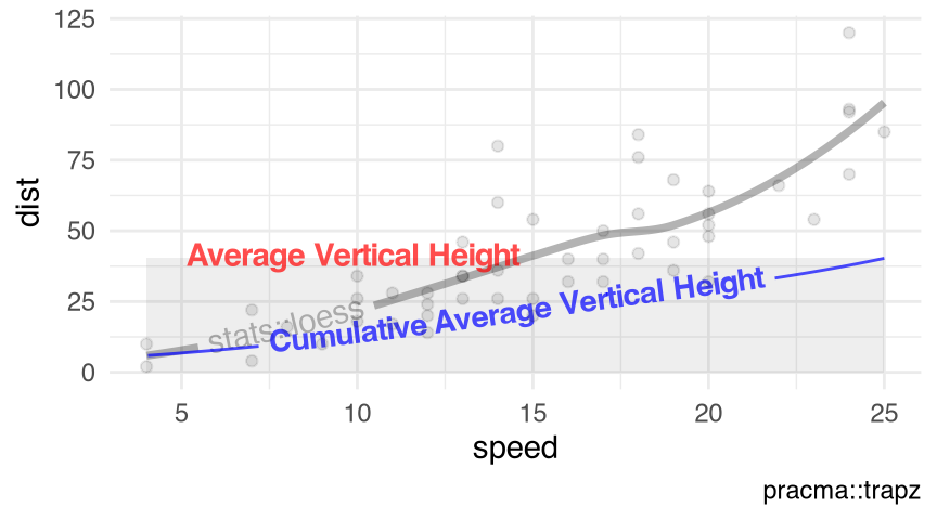
Figure 11.5 visualizes the kernel regression smoother ksmooth() with the numeric response $dist and the numeric predictor $speed in the data set cars (Section 10.7).

Listing 11.13: Figure: function visualize_vtrapz.ksmooth()

datasets::cars |>
  with.default(data = _, expr = {
    ksmooth(x = speed, y = dist, kernel = 'normal', bandwidth = 2)
  }) |> 
  groupedHyperframe:::visualize_vtrapz.ksmooth() + 
  ggplot2::geom_point(
    data = datasets::cars, 
    mapping = ggplot2::aes(x = speed, y = dist), 
    alpha = .1
  ) +
  ggplot2::labs(x = 'speed', y = 'dist')

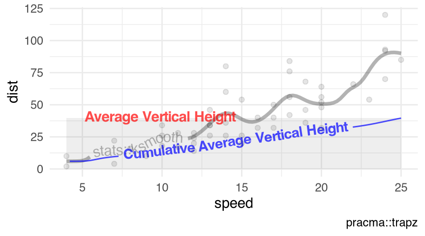
Figure 11.7 visualizes the predicted values of the smoothing spline estimates smooth.spline() with the numeric response $dist and the numeric predictor $speed in the data set cars (Section 10.7).

Listing 11.14: Figure: function visualize_vtrapz.smooth.spline()

datasets::cars |>
  with.default(data = _, expr = smooth.spline(x = speed, y = dist)) |> 
  visualize_vtrapz()

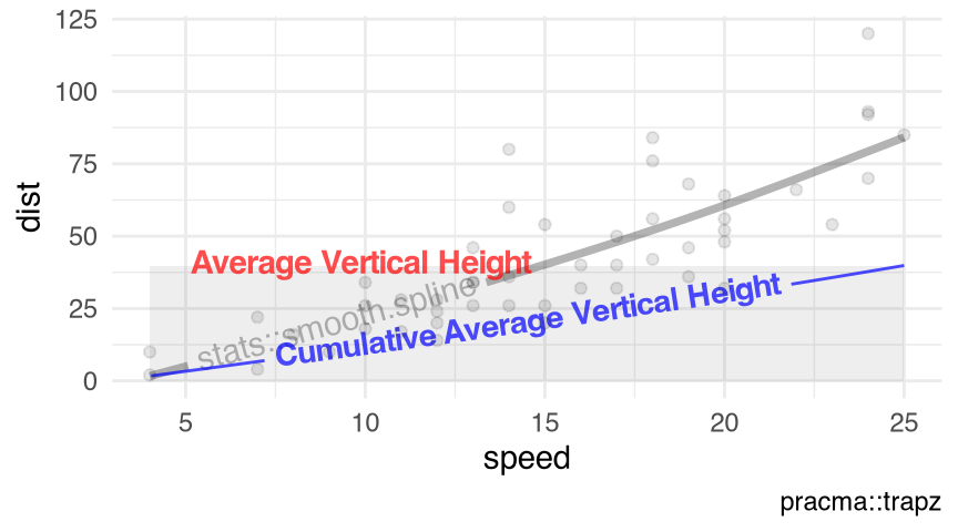
Figure 11.8 visualizes the receiver operating characteristic (ROC) curve of the point-pattern (Baddeley et al. 2025) swedishpines (Section 10.22). Note that

the average vertical height of the trapezoidal integration under the ROC-curve of a point-pattern, via function roc.ppp(); and
the area-under-ROC-curve (AU-ROC) of a point-pattern, via function auc.ppp()

are mathematically equivalent, although not numerically identical (Listing 11.15, as of package spatstat.explore v3.8.0, GPL (>= 2)), because the $x$-domain is $[0,1]$ for an ROC curve.

Listing 11.15: Review: roc.ppp() vs. auc.ppp()

Code

spatstat.data::swedishpines |>
  spatstat.explore::roc.ppp(covariate = 'x') |>
  spatstat.explore::with.fv(expr = {
    vtrapz(x = p, y = raw)
  }) |>
  all.equal.numeric(
    target = _, 
    current = spatstat.data::swedishpines |> 
      spatstat.explore::auc.ppp(covariate = 'x')
  )
# [1] "Mean relative difference: 0.0001160553"

Listing 11.16: Figure: function visualize_vtrapz.fv()

spatstat.data::swedishpines |>
  spatstat.explore::roc.ppp(covariate = 'x') |> 
  visualize_vtrapz()

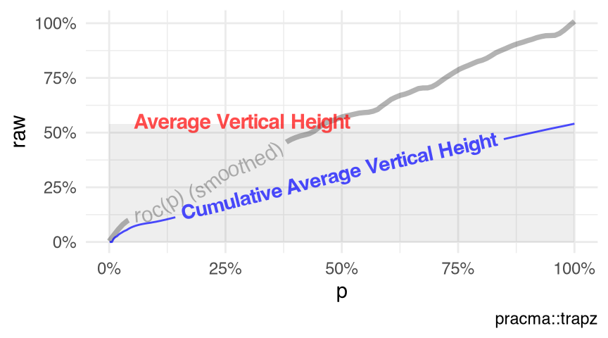
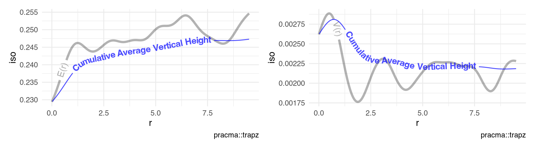
Figure 11.9 visualizes the conditional mean $E(r)$ and variance $V(r)$ between the points and the marks (Schlather et al. 2003) of the point-pattern spruces (Section 10.21) using the functions Emark() and Vmark() (v3.8.0, GPL (>= 2)).

Listing 11.17: Figure: function visualize_vtrapz.listof()

list(
  spatstat.data::spruces |>
    spatstat.explore::Emark(),
  spatstat.data::spruces |>
    spatstat.explore::Vmark() 
) |>
  groupedHyperframe:::visualize_vtrapz.listof(draw.rect = FALSE)